| Back OpEd News | |||||||
|
Original Content at https://www.opednews.com/articles/Two-New-General-Wealth-Equ-by-Mark-Whittington-Capitalism_Capitalism_Capitalism-Failures_Capitalism-Over-Humanity-140317-953.html (Note: You can view every article as one long page if you sign up as an Advocate Member, or higher). |
|||||||
March 17, 2014
Two New General Wealth Equations Suggest a New Definition of Capitalism
By Mark Whittington
Yet more evidence that egregious levels of wealth inequality are numerically built into capitalism itself. Takes the subject out of the mystery realm and puts it into the empirical fact realm. Is this system really fair?
::::::::
Note to the reader: please credit the author when using the following equations, graphs, and tables since this is original material.
A NEW DEFINITION OF CAPITALISM: Capitalism is a monetary system which distributes wealth by a definable distribution raised to a power of a base as determined by rank, where the percentage of those with average wealth and above approximately equals the percentage of those with no wealth and debt. Given constant average wealth and median wealth, both values become trivial compared to the wealth of the very richest as the number of entities in the economy increases. Capitalism creates huge levels of wealth inequality by intrinsic exponentiation as determined by rank.
If poverty is considered lack of wealth, then poverty must be intrinsic to capitalism based on empirical evidence from the Survey of Consumer Finances from 1983 to 2007 as compiled and adjusted by Edward N. Wolff in Recent Trends in Household Wealth in the United States: Rising Debt and the Middle-Class Squeeze---an Update to 2007.
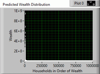
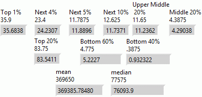
Above is a graph of a hypothetical wealth distribution of an economy of one million households with an average wealth of $369,385 and median wealth of $76,093 using the First General Wealth Equation. The numbers directly above the gray indicators are the actual averaged numbers from the Wolff data from 1983 to 2007. The gray indicators show the computer calculated percentages.
Since the wealth distribution was apparently so skewed, I worked with the natural log of wealth while trying known distributions to describe the data. There were relatively few data points so it was quite a task to either find or create a distribution to fit the data. Eventually I realized the best fit (among commonly used distributions) would be back to back tails of normal distributions as shown in the Natural log of Wealth graph as pictured below:
Entire distribution above is raised as a power to base e to yield the Predicted Wealth Distribution
In order to create a general wealth equation, I believed the equation needed to be scalable in both the wealth and population axes. I found the trick to doing this is taking the famous "Bell Curve" Normal Distribution Probability Distribution Function and modifying it where frequency (people) and probability (wealth) switch axes, where only positive values of wealth are allowed, and where the mean and standard deviation become zero and one respectively to create my First General Wealth Equation:
Wi is an individual's wealth, Ri is the individual's rank either above or below the top 20% in equal decrements in descending order, and A and M are an offset and multiplier respectively.
To evaluate from the top 20% to the wealthiest, use the equation in this form:
To evaluate from the top 20% to the bottom 17.6375%, use the equation in this form:
Where Wa is average wealth, N is the total number of households in the population, and n are integers starting at one and counting away from the top 20%. Households below the bottom 17.6375% have zero wealth.
So using the First General Wealth Equation, one can predict the wealth distribution knowing only average wealth and population size. So in the hypothetical economy of one million households, the evaluation begins above and below the 200,000th richest household in the ranking. Average wealth happens at the 166328th richest household, and zero wealth begins at the 176375th poorest household, making those with average wealth and above at 16.3% approximately equal to those with zero wealth at 17.6% (1.3% difference) considering the entire range of values.
Examining the First General Wealth Equation term,
one can see that as rank decreases (R starts at.398942 and always goes lower for each iteration until the end of the tail is reached), the term increases in value. Depending on the sign of the multiplier M, small linear changes in rank cause large differences in wealth either increasingly or decreasingly since e is being raised to a power which includes rank.
It is worth noting that the multipliers were evaluated using one million members in the economy. If evaluating with a higher number of members, slight adjustment of the multipliers will be necessary.
Almost by accident I noticed that if one takes the log of both the wealth and population axes, and then reverses the axes, a curve much resembling a first order band pass filter (used in electronics)can be seen over the top 80% of the distribution. Here is the Second General Wealth Equation:
The symbol Pw represents the number of households owning wealth and Pi is an individual household starting with the wealthiest at 1 and going to 80% of the population. The bottom 20% when using this equation has no wealth. Taking the log of a predicted Wealth distribution using this equation gives a very similar S shape curve and very similar percentages as compared to the curve of the First General Wealth Equation. The Second General Wealth Equation is also scalable for average wealth and population:
Comparison of First and Second General Wealth Equations. Similar curves produce similar results from independently derived equations.
The Second General Wealth Equation places those with average wealth and above at 18.2% and those with no wealth at 20.0% (1.8% difference) again confirming the approximate equality of the two. Here an exponentiation term with a ratio including rank causes large differences in wealth, although e is not being raised to a power as in the First General Wealth Equation.
If the population is increased above one million, then the exponent (.707) will need to be decreased slightly.
Below are two graphs of Predicted Wealth Distributions using the First General Wealth Equation evaluated with 10,000 entities in the first graph, and then with one million entities in the second graph. Both have approximately equal average and median wealth, but average wealth becomes trivial as the number of entities increases. In a real economy of over one hundred million entities, average wealth is not discernable when graphed with the richest entities.
The First and Second General Wealth Equations will need a slope adjustment if one is concerned with the very top of the distribution. The very top of the distribution is the least predictable in the real world because in either personal wealth or market capitalization the very top tend to break into clusters (shell structure). For some as yet unknown reason the top 26 entities are too high in wealth vs. the empirical data, so adjust the slopes as follows:
Finally, below is a table from Edward N. Wolff's Recent Trends in Household Wealth in the United States: Rising Debt and the Middle-Class Squeeze---an Update to 2007 from which most of the data used in this report was collected. Looking at part A, one can see that under the Percentage Share of Wealth or Income Held by: heading, the percentages have remained fairly constant concerning net worth since reliable data began being collected in 1983. The Bottom 40.0% column shows that near zero wealth has remained constant for decades, implying that something intrinsic to capitalism itself causes systemic, predictable poverty.
Authors Bio:
I am an Automation Programmer and former Congressional candidate who lives in Columbia, SC.


